Thanks for the Band Diagram Tutorial for Quantum ESPRESSO
Dependence
-
Quantum Espresso
-
Python3 + Numpy + Matplotlib
Workflow of band diagram
The procedures in this workflow should use the same outdir and prefix configurations.
pw.x
&control and etc. settings for each procedure:
vc-relax
1
2
&control
    calculation='vc-relax',
scf
1
2
&control
    calculation='scf',
nscf
1
2
&control
    calculation='nscf',
bands
1
2
&control
    calculation='bands',
after CELL_PARAMETERS section, involve
1
2
3
4
5
K_POINTS crystal
    k_points_in_total
    a   b   c   wk
    a   b   c   wk
    a   b   c   wk
The K_POINTS here should follow certain K-path.
The k points settings share the same file coord.txt as in How to Generate QHA Input.
bands.x
The input for bands.x would be like
1
2
3
4
5
&BANDS
  prefix="the_prefix"
  outdir="the_outdir"
  filband="Band.dat"
/
Plot band diagram
Learn about the Quantum ESPRESSO output from bands.x
There are several output types (supposed using filband="Band.dat" in the input for bands.x):
-
Band.dat.gnuwith bands in eV, directly plottable using gnuplot -
Band.dat.rapwith symmetry information, to be read by plotting codeplotband.x` -
Band.datcontaining the band structure, in a format suitable for plotting codeplotband.x -
bandx.out -
scf.outornscf.outProvide the Fermi Energy.
Here, we are using Band.dat to provide band energy, K_Path, and high-symmetry information, scf.out to provide Fermi Energy.
1
2
3
4
5
6
7
8
9
10
11
12
13
14
15
16
17
18
19
20
21
22
23
24
25
26
27
28
29
30
31
32
33
34
35
36
37
38
39
40
41
42
43
44
45
46
47
48
49
50
51
52
53
54
55
56
57

import numpy as np
import matplotlib.pyplot as plt
import os
import re

def dist(a,b):
    # calculate the distance between vector a and b
    d = ((a[0]-b[0]) ** 2 + (a[1]-b[1]) ** 2 + (a[2]-b[2]) ** 2)**0.5
    return d

def read_fermi(file_name):
    # Read the fermi energy in scf.out
    fermi = 0
    with open(file_name, "r") as f:
        lines = f.readlines()
    for line in lines:
        if "the Fermi energy" in line:
            fermi = float(line.split()[4])

    return fermi

def read_bnd(file_name):
    # Read the bands in Band.dat
    coord_regex = r"^\s+(.\d+.\d+)\s+(.\d+.\d+)\s+(.\d+.\d+)$"
    x_coord = []
    x = []
    bands = dict()

    with open(file_name, "r") as f:
        lines = f.readlines()

    for i in range(len(lines)):
        line = lines[i]
        match = re.match(coord_regex,line)
        if match:
            x_coord.append([float(match.group(1)), float(match.group(2)), float(match.group(3)) ])
            bandddd = lines[i+1] + lines[i+2]
            bandddd = bandddd.split()

            for j in range(len(bandddd)):
                if j not in bands.keys():
                    bands[j] = []
                bands[j].append(float(bandddd[j]))
    for i in range(len(x_coord)) :
        if i == 0:
            x.append(0)
        else:
            x.append( x[-1] + dist(x_coord[i], x_coord[i-1]))
    return bands,x

def plot(bands, x, fermi):
    xaxis = [min(x),max(x)]
    for i in bands.values():
        plt.plot(x, i, color=color_dic[pressure], lw=0.2)
    plt.plot(xaxis, [fermi, fermi], color="#66ccff",ls="solid", alpha = 0.5,lw = 1.2)
    plt.xlim(xaxis)
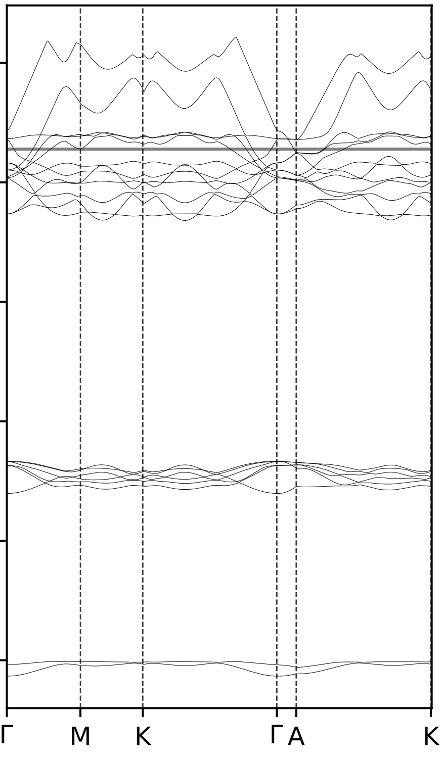
- Plot example: